Most are familiar wit the concept of likelihood ratio tests, or Akaike’s Information criterion for model comparison. This tutorial describes how to compare models using Bayes Factors. These allow comparing nested and un-nested models, without assuming Normality, or large samples. Bayes factors are ratios of marginal likelihoods. In contrast to maximum likelihood, the marginal likelihood is the integral of the likelihood function over the complete parameter range. MIGRATE can calculate such marginal likelihoods for a particular migration model (Beerli and Palczewski 2010). This tutorial steps through all necessary program runs to calculate Bayes factors for comparing different gene flow models. We need to do following:

1. Decide on the models that are interesting for a comparison. The method does not work well for a fishing expedition where one would try to evaluate all models. Only for models with few parameters, for example for three populations, it will be possible to enumerate all models, for more than 3 populations that task will be very daunting.
   

2. Run each model through MIGRATE. Use the same prior settings for each of them because the prior distribution has some influence on the Bayes factors. Use the heating menu to allow for at least four heated chains, use the # menu suggestion for best results, so that the temperatures are spaced so that the inverse of the temperature are regularly spaced on the interval 0 to 1. For example the the 4 different chains have temperatures 1.0, 1.5, 3.0, 100,000.0, this results in the spacing 1.0, 0.666, 0.333, and 0.0.
   

3. Compare the marginal likelihood of the different runs and calculate the Bayes factor and calculate the probability for each model.
   

The following pages detail all steps using a small example. We use a simulated dataset that was generated using parameters that force a direction of migration from the population Aadorf (A) to the population Bern (B). The Bern population is 10x larger than the Aadorf population and no individual from Bern ever goes to Aadorf, but Bern receives about 1 migrant per generation from Aadorf. The dataset name is twoswisstowns. We will evaluate 4 models: (1) a full model with two population sizes and two migration rates (from A to B and from B to A); (2) a model with two population sizes and one migration rate to Bern; (3) a model with two population sizes and one migration rate to Aadorf; (4) a model where Aadorf and Bern are part of the same panmictic population. we know the truth therefore we have some prejudice about the ranking of the models, model 2 should be best, model 1, because it allows the same migration direction as model 2 should be ranked second. Whether model 3 is better than model 4 is unknown a priori and may depend on the strength of the data. First we need to figure out how to run the dataset efficiently in MIGRATE. For that we pick the most complicated model 1 and experiment with run conditions until we are satisfied that the run converges and delivers posterior distributions that look acceptable.

Here are detailed instructions how to rank population genetics models for a particular dataset.

1. 1.Make sure that there is no file called parmfile in the directory you want to run our experiment.
   

2. 2.Start the program MIGRATE-N (I will call it from now on simply MIGRATE). In the Input/Output formats menu change the Datafile name to twoswisstowns, Return to the main menu.
   

3. 3.In the Search strategy menu change the strategy from the default (likelihood) to Bayesian inference. Change the Number of recorded steps in chain to 1000. Do not worry about priors or other runtime options for the moment. Return to the main menu.
   

4. 4.Save the changes by using the menu item write a parmfile.
   

5. 5.Now run the program (pressing Y will start the run if you are in the main menu). For this dataset the runtime will be very short on a modern computer, if this takes more than 1 minute something is not set up correctly. On my computer this takes 5.2 seconds.
   

6. 6.The program writes considerable information during the run to the screen, that gives some information about the run. Most interesting are the acceptance ratio for the genealogy and the autocorrelations of the parameter and the genealogy. The default acceptance method for parameters is Slice sampling (see background information); the acceptance ratio of Slice sampling is always 1.0. If the autocorrelation is high and the effective sample size is low (<500) then a longer run may be needed. If the priors boundaries are to tight, then you will see that the values reported and are either very close or exactly at the upper prior boundary, in these cases you need to extend the prior range. See prior problems, but for this dataset we will have no such problems.
   

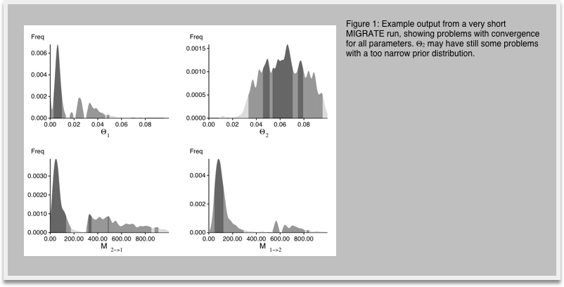
7. 7.Look at the outfile.pdf, you may need a PDF viewer like acroread or Preview.app (on Macintosh computers use open outfile.pdf.  In the outputfile figures labeled Bayesian analysis: Posterior distribution, you see histograms similar to the ones in Figure 1. We expect single peaks where the shading of the histogram shows one  dark block in the center (50% credibility set), two light gray bars indicating the extent of the 95% credibility set, and two lighter gray bars indicating the 99% credibility set.
   

   

   
   
   
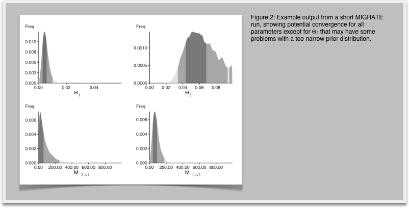
8. 8.In your investigation of Figure 1 you recognize that the histogram does not look very smooth because our run was too short, now restart MIGRATE and set in the strategy menu the setting for change the number of recorded steps in chain from 1,000 to 10,000. This will lengthen the run by a factor of 10. Don't forget to write the parmfile to save the settings. Run and compare the results (Figure 2) with the histogram from before. You will recognize that the longer run has somewhat smoother histograms, and the double peaks vanish (hopefully). With your own data you may want to do another round of refinements, but eventually, by comparing the medians and means of the parameters in the table and the shape of the histograms you should see a good agreement on similar values, if the modes of the different runs are not within the 50% credibility intervals you certainly need to run longer.
   
   

   

   
   
   

9. 9.Let's assume that our runs are all satisfactory. We turn now to the best estimation of the marginal likelihood to compare models. Because we want to use the thermodynamic integration method, we need to turn on heating. Start MIGRATE, use the strategy menu and turn on heating, use static heating. MIGRATE will tell what to do next, you will need to enter 4 chains sampling at every tenth (10) interval using the temperature scheme that is suggested with the character #. Save the parmfile, and run. This will take about 4x longer than before. It should give a better posterior distribution histogram and will add a full table of (natural) log marginal likelihoods is shown towards the end of the outfile.pdf. On my computer this takes about 5 minutes.
   

10. 10. If you are at one of my workshops: Come to the front and write down the log marginal likelihood into the spreadsheet. You will need the numbers from the row labeled All, in the table there are three columns, report the values for the Bezier approximation and the harmonic mean method. (This was our first model, we will compare the different models at the end of this exercise: my log marginal likelihood values for the Bezier approximated score and the Harmonic mean are -4862.85 and -4791.29, respectively.
    

11. 11.Copy the parmfile to parmfile.4param, copy outfile to outfile.4param, and copy outfile.pdf to outfile.4param.pdf
    

12. 12.We start now to work on those other models. We pick the easiest first: mo

    Figure 3: Gene flow model 2 was used to generate the example data.
    

    

     

    del 4. Start MIGRATE and choose the menu Parameter settings.  Choose the entry about sampling locations. We want to use the data as if we would have sampled a single population, therefore we need to claim that the two locations Aadorf and Bern belong to the same panmictic population, this is done by telling MIGRATE that the dataset has two locations (2), and that they are in the same population by using " 1    1". With multiple populations more complicated settings are possible. Run MIGRATE, check the histogram, if it looks OK, come to the front and write down the log marginal likelihoods (again the row labeled All, Bezier and Harmonic score) into the spreadsheet under model 4. My run took 183 seconds and delivered these log marginal likelihoods -4887.25 and -4803.22.
    
13. 13.Copy the parmfile to parmfile.1param, copy outfile to outfile.1param, and copy outfile.pdf to outfile.1param.pdf

    

    
    
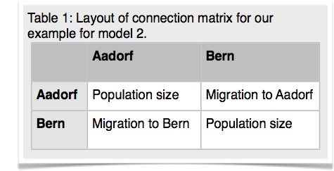
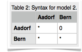
14. 14.Copy the parmfile.4param to parmfile. We want to work now on the remaining two models. Start MIGRATE, choose the parameter menu. Choose the entry labeled Model is set to. MIGRATE will now show a dizzying list of options, don't panic, we will only use few of them. MIGRATE will ask you how many populations are used: enter 2. For a 2-population model we can have 4 parameters. Two population sizes and two migration rates. Before you enter values, please read this whole paragraph. A * or x means that that particular parameter will be estimated, a zero means that that particular parameter will not be estimated (is not used). Our goal is to set one of the migration parameters to zero. We start with model 2 (Figure 3). MIGRATE needs to know how to treat all connections between the populations are specified and that we also give instructions how the program will treat the population sizes. Because we want to estimate both population sizes and one migration rate, w

    

    e will use the * and a zero for the unused migration rate. The connection matrix is square so we can label it like show in the first table below.  MIGRATE asks now that you input each row, this can be done by either specifying * 0 (see second table) and then return and then entering the next line * * return (second row in second table), or you can enter the whole matrix as * 0 * *. Exit the parameter menu, write the parmfile, run MIGRATE, check the histogram, report the log marginal likelihoods. My run took 156 seconds, and delivered these log marginal likelihoods: -4860.58, -4795.88.
    Cautionary note: if you use this tutorial for your own work, please recognize that a standard run in migrate can only use migration model that allow to draw a complete genealogy, so for example a model * 0 0 *, that has no migration among the population, does not work out of the box. As a rule of thumb each population must be connected to at least one other population.
    

15. 15.Copy the parmfile to parmfile.3aparam, copy outfile to outfile.3aparam, and copy outfile.pdf to outfile.3aparam.pdf
    

16. 16.Run model 3 using the same procedure as for model 2. The string for the  migration connection matrix is * * 0 *.  Write parmfile, run, report. My run took 151 seconds and the log marginal likelihoods were -4863.08, and -4794.53.
    

17. 17.Copy the parmfile to parmfile.3bparam, copy outfile to outfile.3bparam, and copy outfile.pdf to outfile.3bparam.pdf
    

18. 18.Once about more than half of the class has reached this point we will talk about the marginal likelihoods found.
    

19. 19.How to calculate Bayes factors? In the Table 3 I summarized all log marginal likelihoods, ln(mL), the Bayes factors are often calculated in very different ways. Here, I report the natural log Bayes factors where
    

Using the guidelines of Kass and Raftery (1995), values smaller than -2 suggest preference for model 2, values larger than 2 suggest preference for model 1. We can use the log marginal likelihoods or the BF to order the models (see column Choice in the Table 3). We also can calculate the model probability. The above outline uses only log marginal likelihoods, for these calculations we need marginal likelihoods. It is calculated by dividing each marginal likelihood by the sum of the marginal likelihoods of all used models:

The calculation of model probabilities from the reported log likelihoods is easy with computer programs that have variable precision (for example Maple or Mathematica). Calculations on a desk calculator often fail, for example the likelihood of model 1 is a remarkable small number because the likelihood is exp(-4862.85)= 1.233 x 10-2112, my emulated HP sci 15C calculator delivers 0.0000. But you can calculate the above quantities using this recipe: (1) find the largest log likelihood (-4860.58), (2) subtract that number form each log likelihood in the list (result: -2.27, 0.0, -2.5, -26.67), (3) exponentiate each element in the new list (result: 0.1033, 1.0, 0.0821, 2.6144 x 10-12) , (4) sum all elements in the list up (0.1033+1.0+0.0821+2.6144 x 10-12), this is the denominator (1.1854). (5) now divide each element in the list by that sum and the numbers will look like the one in table 3 last column.

The harmonic mean fails to recover the true model for my example run and orders the models differently. Often the variance of the harmonic man estimator (when running the same model multiple times) is large. It is therefore not reliable, but this may depend on the dataset. As consequence, I suggest to use the thermodynamic integration method if the extra cost in runtime is acceptable.

Looking at the model probabilities we can see that the “true” model has considerably higher support than the full model or the model that suggests a wrong direction of gene flow.

References

Beerli, P. and M. Palczewski. Unified framework to evaluate panmixia and migration direction among multiple sampling locations. 2010. Genetics 185: 313–326.

Kass, R. E.  and A. E. Raftery. Bayes factors. 1995. Journal of the American Statistical Association 90(430): 773– 795.